The Gradient

We start with a general discussion of functions. A function of two variables is usually written $y=f(x)$ and is a curve in the two dimensional $x, y$ plane. Similarly a function of three variables is usually written $z=f(x, y)$ and is a surface in three dimensional space with $x, y$ and $z$ coordinates. We may think of each point $(x, y)$ in the $x, y$ plane as giving us a unique $z$ which is the height of the surface above that point. What about a function for four variables $\phi=f(x, y, z)$? This is a hypersurface in four dimensional space but we can get an intuitive mental picture of it as follows. We only have to think of $x, y, z$ as the coordinates of a random point in a room and $\phi$ as the temperature at that point. Every single point in the three dimensional room have a set of coordinates $(x, y, z)$. We put these coordinates in the function and out comes $\phi$ the temperature at that point!

Now suppose we pick some random point A in the room and find the temperature $\phi$ there. If we move away from A by a short distance $ds$ in the direction of the unit vector $\hat{\mathbf{u}}$ the temperature will change by $d\phi$. We now try to calculate this change.

Since

$$\mathbf{ds}=ds\hat{\mathbf{u}}=dx\hat{\mathbf{i}}+dy\hat{\mathbf{j}}+dz\hat{\mathbf{k}}$$

we break the movement by $ds$ in the direction of $\hat{\mathbf{u}}$ into three steps. First we move by an amount $dx$ in the $x$ direction. Since the $y$ and $z$ coordinates remain fixed the change in temperature is given by

$$d\phi_x=\frac{\partial\phi}{\partial x}dx$$

Similarly when we move by an amount $dy$ parallel to the $y$ axis the temperature change is

$$d\phi_y=\frac{\partial\phi}{\partial y}dy$$

Finally when we move by a step $dz$ parallel to the $z$ axis the temperature change is

$$d\phi_z=\frac{\partial\phi}{\partial z}dz$$

Adding these three changes together we find the total change is

$$d\phi=\frac{\partial\phi}{\partial x}dx+\frac{\partial\phi}{\partial y}dy+\frac{\partial\phi}{\partial z}dz$$

we may write this as a dot product

$$d\phi=\left(\frac{\partial\phi}{\partial x}\hat{\mathbf{i}}+\frac{\partial\phi}{\partial y}\hat{\mathbf{j}}+\frac{\partial\phi}{\partial z}\hat{\mathbf{k}}\right)\cdot\left(dx\hat{\mathbf{i}}+dy\hat{\mathbf{j}}+dz\hat{\mathbf{k}}\right)$$

The expression in the first set of parentheses is called the gradient of $\phi$ sometimes written as grad$\phi$. We may think of the expression

$$\frac{\partial}{\partial x}\hat{\mathbf{i}}+\frac{\partial}{\partial y}\hat{\mathbf{j}}+\frac{\partial}{\partial z}\hat{\mathbf{k}}$$

as an operator which acts on $\phi$ to give the gradient. This vector differential operator is represented by the symbol $\nabla$ which is called del or sometimes nabla after an ancient Phoenician harp it apparently resembles. Some see it as an inversion of the Greek letter delta $\Delta$ and call it atled which is delta spelled backwards. We may now write our equation for the change in temperature compactly as

$$d\phi=\nabla\phi\cdot\hat{\mathbf{ds}}$$

The rate of change of the temperature with distance in the direction of the unit vector $\hat{\mathbf{u}}$ is now given by

$$\frac{d\phi}{ds}=\nabla\phi\cdot\frac{\hat{\mathbf{ds}}}{ds}=\nabla\phi\cdot\hat{\mathbf{u}}$$

If we call the angle between our chosen unit vector $\hat{\mathbf{u}}$ and the gradient vector $\theta$ then we can evaluate the dot product as

$$\frac{d\phi}{ds}=|\nabla\phi|\cos\theta$$

This formula gives us a wealth of information about the gradient vector. All we have to do is consider the case of $\theta=0$ meaning that our chosen unit vector $\hat{\mathbf{u}}$ points in the direction of the gradient vector. Then $\cos\theta$ has its maximum value of one and $\frac{d\phi}{ds}$ has its maximum value of $|\nabla\phi|$. Thus the gradient vector points in the direction in which the field changes most rapidly with distance and the magnitude of the gradient vector is this maximum rate of change.

We now introduce the idea of level surfaces for which $\phi=f(x,y,z)$ is a constant. Everywhere on a level surface $\phi$ takes the same value. If the field values represent temperature (pressure) they are termed isotheral (isobaric) surfaces. If we consider small enough portions of such surfaces then they are essentially flat. Fig. 1 shows two such surfaces in close proximity i.e. $\phi=C$ and $\phi=C+dC$

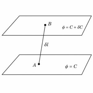
Fig. 1. Level Surfaces

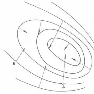
Fig. 2. Level Lines and Gradients

The rate of change of the field is given by

$$\frac{d\phi}{ds}\approx\frac{\delta C}{\delta l}$$

So the rate of change is greatest when $\delta l $ is smallest i.e when AB is perpendicular to the surfaces. This implies that the gradient vector is perpendicular to the level surfaces. Also when $\delta l$ is small or the level surfaces are close together the gradient is large. Conversely when $\delta l$ is large or the level surfaces are far apart the gradient is small.

In two dimensions we speak of level lines instead of level surfaces. Fig. 2. shows the contour map of a hill. On any line all points are at the same height above sea level. Gradient vectors are shown at points A and B can be seen to be perpendicular to the level lines. At A where the lines are close together the vector is long. This means the gradient is large where the hill is steep and a small shift in position means a large change in height. At B where the lines are spaced far apart the vector is short. This means the gradient is small where the hill gently slopes and a small change in position means a small change in height.

As an example in calculating the gradient consider the following scalar function

$$\phi=\phi(x, y, z)=x$$

At any point $(x, y, z)$ the value of $\phi$ does not depend on $y$ or $z$. Thus in any plane parallel to the $yz$ plane $\phi$ is constant and equal to the $x$ coordinate of the point where that plane cuts the $x$-axis. This means the level surfaces are planes parallel to the $yz$ plane and the gradient vector is perpendicular to the $yz$ plane and hence parallel to the unit vector $\hat{\mathbf{i}}$. The fact that the rate at which the field increases with distance in the $x$ direction is one means that the magnitude of the gradient is also one. Putting together the magnitude and direction we construct the gradient vector as $\hat{\mathbf{i}}$. Below we give a formal calcaulation showing that this is indeed correct.

$$\nabla x=\frac{\partial x}{\partial x}\hat{\mathbf{i}}+\frac{\partial x}{\partial y}\hat{\mathbf{j}}+\frac{\partial x}{\partial z}\hat{\mathbf{k}}=1\hat{\mathbf{i}}+0\hat{\mathbf{j}}+0\hat{\mathbf{k}}=\hat{\mathbf{i}}$$

As a more interesting example in computing the gradient we turn to the scalar field

$$\phi=f(r)$$

where

$$r=(x^2+y^2+z^2)^{\frac{1}{2}}$$

This field is spherically symmetric and the level surfaces are spheres centered on the origin. The gradient is perpendicular to these spheres and hence lies parallel to the unit radial vector $\hat{\mathbf{r}}$. Now the rate at which $\phi$ increases with distance from the origin is $\frac{df}{dr}$. This is the magnitude of the gradient. Putting together the magnitude and direction we can construct gradient vector as $\frac{df}{dr}\hat{\mathbf{r}}$. Again we show that this is correct by formal calculation

$$\frac{f(r)}{\partial x}=\frac{df}{dr}\frac{\partial r}{\partial x}=\frac{df}{dr}\frac{1}{2}(x^2+y^2+z^2)^{\mathbin{-}\frac{1}{2}}\cdot 2x=\frac{df}{dr}\frac{x}{(x^2+y^2+z^2)^{\frac{1}{2}}}=\frac{df}{dr}\frac{x}{r}$$

in exactly the same way we can calculate

$$\frac{f(r)}{\partial y}=\frac{df}{dr}\frac{y}{r}$$

and

$$\frac{f(r)}{\partial z}=\frac{df}{dr}\frac{z}{r}$$

Thus we have

$$\nabla f(r)=\frac{df}{dr}\frac{x}{r}\hat{\mathbf{i}}+\frac{df}{dy}\frac{y}{r}\hat{\mathbf{j}}+\frac{df}{dr}\frac{x}{r}\hat{\mathbf{k}}=\frac{df}{dr}\frac{x\hat{\mathbf{i}}+y\hat{\mathbf{j}}+z\hat{\mathbf{k}}}{r}=\frac{df}{dr}\frac{\mathbf{r}}{r}=\frac{df}{dr}\hat{\mathbf{r}}$$

This formula has two very special cases which we give below and which you can check by direct calculation if you like.

$$\nabla r=\hat{\mathbf{r}}$$

$$\nabla\frac{1}{r}=\mathbin{-}\frac{1}{r^2}\hat{\mathbf{r}}$$