The Euler-Lagrange Equation

Suppose we have a function $f(x, y, z)$ of three variables given by

$$f(x, y, z)= x^2+y^2+z^2$$

We can use this function to build a machine $J$ that takes in any function $y(x)$ as input and outputs a number. $J$ is called a functional and is given by

$$J[y(x)]=\int_{x_1}^{x_2}f(x, y(x), y^{\prime}(x))dx$$

Let us now show that if we put the function $y=x^2$ into the functional $J$ it really does output a single number. We have

$$y(x)=x^2$$

$$y^{\prime}=2x$$

$$f(x, y, z)=x^2+y^2+z^2$$

$$f(x, y(x), y^{\prime}(x))=x^2+(x^2)^2+(2x)^2=x^4+5x^2$$

So we see that $f$ is really a function of one variable namely $x$ but it is expressed in a complicated way through $y$ and $y^{\prime}$ which both depend exclusively on $x$. Next we calculate the functional

$$J[y=x^2]=\int_{x_1}^{x_2}(x^4+5x^2)dx=\left[\frac{x^5}{5}+\frac{5x^3}{3}\right]_{x_1}^{x_2}=\frac{x_2^5\mathbin{-}x_1^5}{5}+\frac{5(x_2^3\mathbin{-}x_1^3)}{3}=\text{number Q.E.D.}$$

The problem of the calculus of variation is to find the input function $y(x)$ joining the points $(x_1, y_1=y(x_1)),(x_2,y_2=y(x_2))$ for which the functional $J[y(x)]$ is stationary (minimum, maximum or point of inflection). We call $y(x)$ the stationary path and consider a nearby slightly different but non-stationary path $Y(x)$ given by

$$Y(x)=y(x)+\alpha\eta(x)$$

These two paths are shown in Fig. 1 below

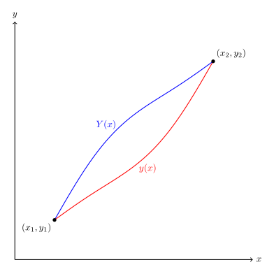
Fig. 1 Stationary red path and non-stationary blue path

Note that

$$y_1=y(x_1)=Y(x_1)\text{ implies that }\eta(x_1)=0$$

$$y_2=y(x_2)=Y(x_2\text{ implies that }\eta(x_2)=0$$

Since $J[Y(x)]$ is a function of $\alpha$ we write

$$J[y(Y(x)](\alpha)=\int_{x_1}^{x_2}f(Y,Y^{\prime},x)dx$$

Now when $\alpha=0$

$$Y(x)=y(x)+\alpha\eta(x)=y(x)+0=y(x)$$

i.e. Y(x) is stationary which means that

$$\frac{d}{d\alpha}J[Y(x)](\alpha)|_{\alpha=0}=0$$

Using the chain rule to differentiate $J$ with respect to $\alpha$ we get

$$\frac{d}{d\alpha}J[Y(x)](\alpha)=\int_{x_1}^{x_2}\frac{\partial}{\partial\alpha}f(Y,Y^{\prime},x)=\int_{x_1}^{x_2}\left(\frac{\partial f}{\partial Y}\frac{dY}{d\alpha}+\frac{\partial f}{\partial Y^{\prime}}\frac{dY^{\prime}}{d\alpha}\right)dx$$

Applying the $\alpha=0$ condition that makes the path stationary we get

$$\begin{aligned}0&=\int_{x_1}^{x_2}\left(\eta(x)\frac{\partial f}{\partial y}+\eta^{\prime}(x)\frac{\partial f}{\partial y^{\prime}}\right)dx\\&=\int_{x_1}^{x_2}\left(\eta(x)\frac{\partial f}{\partial y}\mathbin{-}\eta(x)\frac{d}{dx}\frac{\partial f}{\partial y^{\prime}}\right)dx+\left[\eta(x)\frac{\partial f}{\partial y^{\prime}}\right]_{x_1}^{x_2}\\&=\int_{x_1}^{x_2}\eta(x)\left(\frac{\partial f}{\partial y}\mathbin{-}\frac{d}{dx}\frac{\partial f}{\partial y^{\prime}}\right)dx\end{aligned}$$

Where we used integration by parts. The fact that $\eta(x)$ is zero at the endpoints $x_1$ and $x_2$ means that the boundary term in square brackets is zero. We conclude that the expression in parenthesis is zero for all $x$ and this gives the Euler-Lagrange Equation

$$\frac{d}{dx}\frac{\partial f}{\partial y^{\prime}}\mathbin{-}\frac{\partial f}{\partial y}=0$$

The steps involved in using this equation are

Step 1: You are given a real-world problem typically of the form “Which curve y(x) satisfies some extremal condition”

Step 2: Find the integral $J$ that must be made stationary

Step 3: From the integral extract the function $f$

Step 4: Use $f$ to write and then solve the Euler-Lagrange Equation

Step 5: The solution gives the required curve $y(x)$