We start with the evaluation of an improper definite integral using integration by parts

$$I_n=\int_0^\infty x^n e^{\mathbin{-}ax}dx=\int_0^\infty x^n\frac{d}{dx}\left(\mathbin{-}\frac{1}{a}e^{-ax}\right)dx=\left[\mathbin{-}\frac{1}{a}x^n e^{\mathbin{-}ax}\right]_0^\infty+\frac{1}{a}\int_0^\infty e^{\mathbin{-}ax}\frac{d}{dx}x^n dx$$

The term in square brackets is called the boundary term because we evaluate it at the boundaries zero and infinity. It is conveniently zero because:

(i) at $x=0, x^ne^{\mathbin{-}ax}=0^ne^0=0\cdot1=0$

(ii) at $x=\infty$ we may think of $x$ as growing arbitrarily large. Since the decaying exponential decreases faster than the growth of any power of $x$ then $\lim_{n\to\infty}x^ne^{\mathbin{-}ax}=0$

Thus we can drop the boundary term entirely and write

$$I_n=\frac{1}{a}\int_0^\infty e^{\mathbin{-}ax}nx^{n\mathbin{-}1}dx=\frac{n}{a}I_{n\mathbin{-}1}$$

This is our recursion relation and we apply it repeatedly until we get the integral $I_0$ that we can easily evaluate. 

$$I_n=\frac{n}{a}I_{n\mathbin{-}1}=\frac{n}{a}\frac{n\mathbin{-}1}{a}I_{n\mathbin{-}1}\cdots=\frac{n(n\mathbin{-}1)\cdots(n\mathbin{-}(n\mathbin{-}1))}{a^n}I_{n\mathbin{-}n}=\frac{n!}{a^n}I_0=\frac{n!}{a^n}\int_0^\infty e^{\mathbin{-}ax}dx=\frac{n!}{a^n}\left[\frac{1}{a}e^{\mathbin{-}ax}\right]_0^\infty$$

Finally we have a very nice result

$$\int_0^\infty x^n e^{\mathbin{-}ax}dx=\frac{n!}{a^{n+1}}$$

Just for fun we evaluate this integral using a different method. We start with

$$\int_0^\infty e^{\mathbin{-}ax}dx=\left[\mathbin{-}\frac{1}{a}e^{\mathbin{-}ax}\right]_0^\infty=\frac{1}{a}$$

Next we differentiate this with respect to $a$ (treating $x$ as a constant) to get

$$\int_0^\infty\mathbin{-}xe^{\mathbin{-}ax}dx=\mathbin{-}\frac{1}{a^2}$$

We discard the minus signs from both sides and differentiate again to get

$$\int_0^\infty\mathbin{-}x^2e^{\mathbin{-}ax}dx=\mathbin{-}\frac{2}{a^3}$$

doing this once again we get

$$\int_0^\infty \mathbin{-}x^3e^{\mathbin{-}ax}dx=\mathbin{-}\frac{2\cdot 3}{a^4}$$

Continuing the above procedure we see that for any positive integer $n=1,2,3,4…$

$$\int_0^\infty x^ne^{\mathbin{-}ax}=\frac{n!}{a^{n+1}}$$

Now setting $a=1$ gives

$$\int_0^\infty x^ne^{\mathbin{-}x}=n!$$

Setting $n=0$ we can evaluate the integral to show that $0!=1$. However we can do something more interesting. Suppose we evaluate the integral for $n=\frac{1}{2}$. Then the value we get is apparently the factorial of one half! Thus the integral provides a way to extend the factorial functions from positive integers to all real (or indeed complex) numbers. This is done by the gamma function which is defined as

$$\Gamma(p)=\int_0^\infty x^{p\mathbin{-}1}e^{\mathbin{-}x}dx$$

For $p>0$ this integral converges but for $p\leq 0$ the integral diverges. We now deduce a very important relation from the definition of the gamma function

$$\Gamma(p+1)=\int_0^\infty x^pe^{\mathbin{-}x}dx=\int_0^\infty x^p\frac{d}{dx}\left(\mathbin{-}e^{\mathbin{-}x}\right)dx=\left[\mathbin{-}x^pe^{-x}\right]_0^\infty+\int_0^\infty e^{\mathbin{-}x}\frac{d}{dx}x^pdx=p\int_0^\infty x^{p\mathbin{-}1}e^{\mathbin{-}x}dx=p\Gamma(p)$$

Thus 

$$\Gamma(p+1)=p\Gamma(p)$$

This is the functional equation of the Gamma function. It is also called the recurrence relation of gamma function – a name that is appropriate because it lets you calculate $\Gamma(p+1)$ from $\Gamma(p)$. We also have the rearranged recursion relation

$$\Gamma(p)=\frac{\Gamma(p+1)}{p}$$

This is used to find $\Gamma(p)$ from $\Gamma(p+1)$. Now let us calculate $\Gamma(1)$

$$\Gamma(1)=\int_0^\infty e^{\mathbin{-}x}dx=\left[\mathbin{-}e^{\mathbin{-}x}\right]_0^\infty=\left[e^{\mathbin{-}x}\right]_0^\infty=e^{\mathbin{-}0}\mathbin{-}e^{\mathbin{-}\infty}=1\mathbin{-}0=1$$

Using this result with our recurrence relation we can find the gamma function at higher values in steps of one.

$$\Gamma(2)=\Gamma(1+1)=1\Gamma(1)=1$$

$$\Gamma(3)=\Gamma(2+1)=2\Gamma(2)=2\cdot1$$

$$\Gamma(4)=\Gamma(3+1)=3\Gamma(3)=3\cdot2\cdot1$$

$$\Gamma(5)=\Gamma(4+1)=4\Gamma(4)=4\cdot3\cdot2\cdot1$$

Similarly we can use our rearranged recursion relation and $\Gamma(1)=1$ to find the gamma function at lower values in steps of one.

$$\Gamma(0)=\frac{\Gamma(0+1)}{\Gamma(1)}=\frac{\Gamma(1)}{\Gamma(0)}=\frac{1}{0}=\text{undefined}$$

$$\Gamma(\mathbin{-}1)=\frac{\Gamma(\mathbin{-}1+1)}{\mathbin{-}1}=\frac{\Gamma(0)}{\mathbin{-}1}=\text{undefined}$$

$$\Gamma(\mathbin{-}2)=\frac{\Gamma(\mathbin{-}2+1)}{\mathbin{-}2}=\frac{\Gamma(\mathbin{-}1)}{\mathbin{-}2}=\text{undefined}$$

Thus we can write

$$\Gamma(n)=\begin{cases}(n\mathbin{-}1)!&n=1,2,3,4…\\\text{undefined}&n=0,\mathbin{-}1,\mathbin{-}2,\mathbin{-}3…\end{cases}$$

We state without proof Euler’s reflection formula

$$\Gamma(p)\Gamma(1\mathbin{-}p)=\frac{\pi}{\sin\pi p}$$

Setting $p=\frac{1}{2}$ we easily see that

$$\Gamma(\frac{1}{2})=\sqrt{\pi}$$

Using this result with the recurrence relation we can find gamma at any positive half integer as shown below

$$\Gamma(1.5)=\Gamma(0.5+1)=0.5\Gamma(0.5)=\frac{1}{2}\sqrt{\pi}$$

$$\Gamma(2.5)=\Gamma(1.5+1)=1.5\Gamma(1.5)=\frac{3}{2}\times\frac{1}{2}\sqrt{\pi}$$

$$\Gamma(3.5)=\Gamma(2.5+1)=2.5\Gamma(2.5)=\frac{5}{2}\times\frac{3}{2}\times\frac{1}{2}\sqrt{\pi}$$

and in general for $n=1,2,3,…$ we have

$$\Gamma\left(n\mathbin{-}\frac{1}{2}\right)=\frac{(2n\mathbin{-}3)(2n\mathbin{-}5)\cdots5\times3\times1}{2^{n\mathbin{-}1}}\sqrt{\pi}=\frac{(2n\mathbin{-}3)!!}{2^{n\mathbin{-}1}}\sqrt{\pi}$$

Where we made use of the double factorial notation. Using the rearranged recurrence relation with $\Gamma(\frac{1}{2})=\sqrt{2}$ we can find $\Gamma(\mathbin{-}0.5)$, $\Gamma(\mathbin{-}1.5)$, $\Gamma(\mathbin{-}2.5)$ etc. as shown below

$$\Gamma(\mathbin{-}0.5)=\frac{\Gamma(0.5)}{\mathbin{-}0.5}=\mathbin{-}2\sqrt{\pi}$$

$$\Gamma(\mathbin{-}1.5)=\frac{\Gamma(\mathbin{-}0.5)}{\mathbin{-}1.5}=\mathbin{-}\frac{2}{3}\times\mathbin{-}2\sqrt{\pi}$$

$$\Gamma(\mathbin{-}2.5)=\frac{\Gamma(\mathbin{-}1.5)}{\mathbin{-}2.5}=\mathbin{-}\frac{2}{5}\times\mathbin{-}\frac{2}{3}\times\mathbin{-}2\sqrt{\pi}$$

Note the signs alternate $\Gamma(\mathbin{-}0.5)$ is negative, $\Gamma(\mathbin{-}1.5)$ is positive, $\Gamma(\mathbin{-}2.5)$ is negative etc. In general for $n=1,2,3,4…$ we have

$$\Gamma\left(\frac{1}{2}\mathbin{-}n\right)=(\mathbin{-}1)^n\frac{2^{n\mathbin{-}1}}{(2n\mathbin{-}1)!!}\sqrt{\pi}$$

This technique can be used to evaluate the gamma function at any real number. Thus using numerical integration, tables, software or ai we can find for example that

$$\Gamma(0.3)=\int_0^\infty x^{\mathbin{-}0.7}e^{\mathbin{-}x}dx=2.991569. . .$$

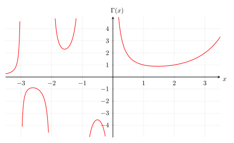
Then using the recurrence relation we can find gamma at $1.3, 2.3, 3.3, 4.3…$ and using the rearranged recurrence relation we can find gamma at $\mathbin{-}0.7$, $\mathbin{-}1.7$, $\mathbin{-}2.7$, $\mathbin{-}3.7$ etc. If we then repeat the entire process several times starting with different numbers between zero and one we will find the value of $\Gamma(p)$ at enough values to allow us to draw the curve shown in Fig. 1.